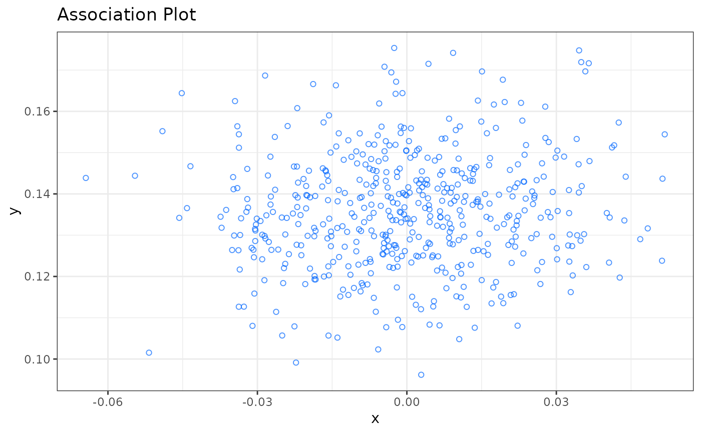
Association Plot

Plot an Association Plot for the chosen columns.

Usage

apl(
  caobj,
  type = "ggplot",
  rows_idx = NULL,
  cols_idx = caobj@group,
  row_labs = FALSE,
  col_labs = FALSE,
  show_score = FALSE,
  show_cols = FALSE,
  show_rows = TRUE,
  score_cutoff = 0,
  score_color = "rainbow"
)

Arguments

caobj

An object of class "cacomp" and "APL" with apl coordinates calculated.

type

"ggplot"/"plotly". For a static plot a string "ggplot", for an interactive plot "plotly". Default "ggplot".

rows_idx

numeric/character vector. Indices or names of the rows that should be labelled. Default NULL.

cols_idx

numeric/character vector. Indices or names of the columns that should be labelled. Default is only to label columns making up the centroid: caobj@group.

row_labs

Logical. Whether labels for rows indicated by rows_idx should be labeled with text. Default TRUE.

col_labs

Logical. Whether labels for columns indicated by cols_idx shouls be labeled with text. Default FALSE.

show_score

Logical. Whether the S-alpha score should be shown in the plot.

show_cols

Logical. Whether column points should be plotted.

show_rows

Logical. Whether row points should be plotted.

score_cutoff

Numeric. Rows (genes) with a score >= score_cutoff will be colored according to their score if show_score = TRUE.

score_color

Either "rainbow" or "viridis".

Value

Either a ggplot or plotly object.

Details

For an interactive plot type="plotly" can be chosen, otherwise a static plot will be returned. The row and column coordinates have to be already calculated by `apl_coords()`.

References

Association Plots: Visualizing associations in high-dimensional correspondence analysis biplots
Elzbieta Gralinska, Martin Vingron
bioRxiv 2020.10.23.352096; doi: https://doi.org/10.1101/2020.10.23.352096

Examples

set.seed(1234)

# Simulate counts
cnts <- mapply(function(x){rpois(n = 500, lambda = x)},
               x = sample(1:100, 50, replace = TRUE))
rownames(cnts) <- paste0("gene_", 1:nrow(cnts))
colnames(cnts) <- paste0("cell_", 1:ncol(cnts))

# Run correspondence analysis
ca <- cacomp(obj = cnts, princ_coords = 3)
#> Warning: 
#> Parameter top is >nrow(obj) and therefore ignored.
#> No dimensions specified. Setting dimensions to: 9

# Calculate APL coordinates for arbitrary group
ca <- apl_coords(ca, group = 1:10)

# plot results
# Note:
# Due to random gene expression & group, no highly
# associated genes are visible.
apl(ca, type = "ggplot")