Runs elbow method
elbow_method.RdHelper function for pick_dims() to run the elbow method.
Arguments
- obj
A "cacomp" object as outputted from `cacomp()`
- mat
A numeric matrix. For sequencing a count matrix, gene expression values with genes in rows and samples/cells in columns. Should contain row and column names.
- reps
Integer. Number of permutations to perform when choosing "elbow_rule".
- python
A logical value indicating whether to use singular value decomposition from the python package torch. This implementation dramatically speeds up computation compared to `svd()` in R.
- return_plot
TRUE/FALSE. Whether a plot should be returned when choosing "elbow_rule".
Value
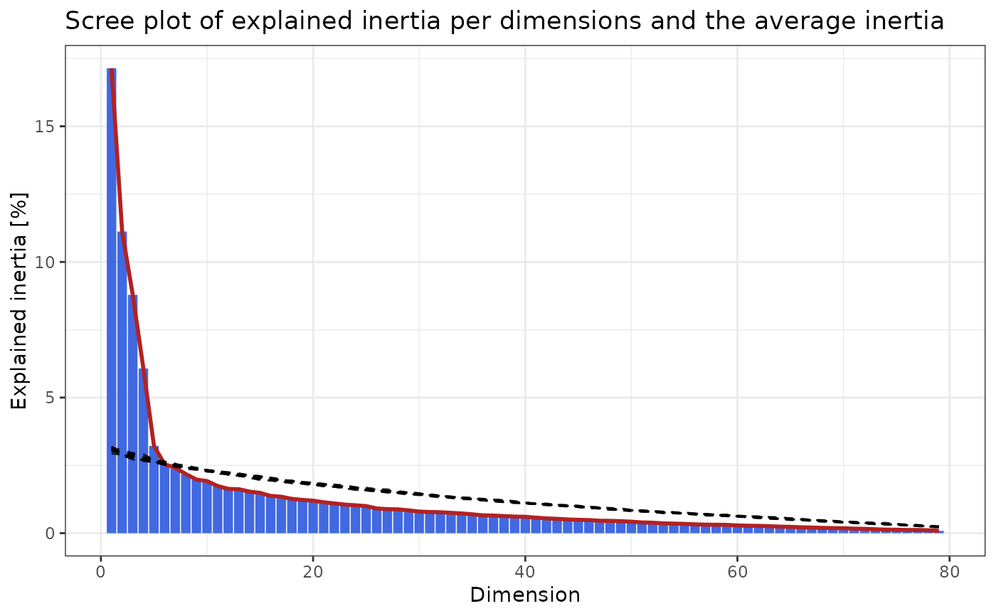
`elbow_method` (for `return_plot=TRUE`) returns a list with two elements: "dims" contains the number of dimensions and "plot" a ggplot. if `return_plot=TRUE` it just returns the number of picked dimensions.
References
Ciampi, Antonio, González Marcos, Ana and Castejón Limas, Manuel.
Correspondence analysis and 2-way clustering. (2005), SORT 29(1).
Examples
# Get example data from Seurat
library(SeuratObject)
set.seed(2358)
cnts <- as.matrix(SeuratObject::LayerData(pbmc_small,
                                          assay = "RNA",
                                          layer = "data"))
# Run correspondence analysis.
ca <- cacomp(obj = cnts)
#> Warning:
#> Parameter top is >nrow(obj) and therefore ignored.
#> No dimensions specified. Setting dimensions to: 15

# pick dimensions with the elbow rule. Returns list.
pd <- pick_dims(obj = ca,
                mat = cnts,
                method = "elbow_rule",
                return_plot = TRUE,
                reps = 10)
#>
  |
  |                                                                      |   0%
  |
  |=======                                                               |  10%
  |
  |==============                                                        |  20%
  |
  |=====================                                                 |  30%
  |
  |============================                                          |  40%
  |
  |===================================                                   |  50%
  |
  |==========================================                            |  60%
  |
  |=================================================                     |  70%
  |
  |========================================================              |  80%
  |
  |===============================================================       |  90%
  |
  |======================================================================| 100%
pd$plot

ca_sub <- subset_dims(ca, dims = pd$dims)