Visualizing and Biclustering scRNA-seq data with CAbiNet
Clemens Kohl (contributed equally)
Max Planck Institute for Molecular Genetics, Berlin, Germanykohl@molgen.mpg.de
Yan Zhao (contributed equally)
Max Planck Institute for Molecular Genetics, Berlin, Germanyzhao@molgen.mpg.de
Martin Vingron
Max Planck Institute for Molecular Genetics, Berlin, Germanyvingron@molgen.mpg.de
CAbiNet.RmdAbstract
CAbiNet allows fast and robust biclustering of ‘marker’ genes and cells in single-cell RNA sequencing (scRNA-seq) data analysis through Correspondence Analysis. The cells and genes together with the biclustering results can be simultaneously displayed in a planar space, the biMAP. CAbiNet can facilitate the cell type annotation of scRNA-seq analysis.
Introduction
CAbiNet allows to jointly visualize cells and genes from scRNA-seq data in a single planar plot, called biMAP. CAbiNet performs biclustering to identify cell groups and their corresponding marker genes, which can be conveniently displayed in the biMAP.
For a more in-depth explanation of CAbiNet, please refer to the pre-print on bioRxiv: https://doi.org/10.1101/2022.12.20.521232
If you are working with CAbiNet please cite:
Zhao, Y., Kohl, C., Rosebrock, D., Hu, Q., Hu, Y., Vingron, M.,
CAbiNet: Joint visualization of cells and genes based on a gene-cell graph.
2022, bioRxiv, https://doi.org/10.1101/2022.12.20.521232
Installation
You can install the package from GitHub by running:
# Until changes are merged into the Bioconductor version, please install the below version of APL.
devtools::install_github("VingronLab/APL", ref = "cabinet-freeze")
devtools::install_github("VingronLab/CAbiNet")
CAbiNet also has a number of python dependencies, namely umap-learn, numpy, pytorch, scikit-learn and scipy. They should be installed automatically during the installation of CAbiNet. If there is an issue, you can also install them manually by running the following:
library(reticulate)
install_miniconda()
use_condaenv(
  condaenv = file.path(miniconda_path(), "envs/r-reticulate"),
  required = TRUE
)

conda_install(envname = "r-reticulate", packages = "numpy")
conda_install(envname = "r-reticulate", packages = "pytorch")
conda_install(envname = "r-reticulate", packages = "scikit-learn")
conda_install(envname = "r-reticulate", packages = "umap-learn")
conda_install(envname = "r-reticulate", packages = "scipy")
If you run into any problem when installing and running our package, please let us know by opening an issue on our GitHub repository https://github.com/VingronLab/CAbiNet/issues. We will help you to solve the problem as best as we can.
Analyzing data with CAbiNet
CAbiNet is designed to work with a count matrix as input, but is also
fully compatible with SingleCellExperiment
objects. We will demonstrate here on the Zeisel Brain Dataset obtained
from the scRNAseq
package how to work with our algorithm and package. This dataset is in a
SingleCellExperiment
(SCE) object format. If you are working with Seurat object, you
can still use it as input to cacomp function from APL.
In the examples below we will prepare the data and then use CAbiNet to bicluster and visualize the cells and their marker genes. We will further use the biMAP and the biclustering information to quickly and easily annotate the cell types.
Setup
Loading the data:
sce <- ZeiselBrainData()
#> snapshotDate(): 2022-04-26
#> see ?scRNAseq and browseVignettes('scRNAseq') for documentation
#> loading from cache
#> see ?scRNAseq and browseVignettes('scRNAseq') for documentation
#> loading from cache
#> see ?scRNAseq and browseVignettes('scRNAseq') for documentation
#> loading from cache
#> snapshotDate(): 2022-04-26
#> see ?scRNAseq and browseVignettes('scRNAseq') for documentation
#> loading from cache
sce
#> class: SingleCellExperiment
#> dim: 20006 3005
#> metadata(0):
#> assays(1): counts
#> rownames(20006): Tspan12 Tshz1 ... mt-Rnr1 mt-Nd4l
#> rowData names(1): featureType
#> colnames(3005): 1772071015_C02 1772071017_G12 ... 1772066098_A12
#>   1772058148_F03
#> colData names(10): tissue group # ... level1class level2class
#> reducedDimNames(0):
#> mainExpName: endogenous
#> altExpNames(2): ERCC repeat
Data pre-processing
CAbiNet is based on Correspondence Analysis, which is sensitive to outliers in the count matrix. We therefore strongly suggest to pre-process your data before applying CAbiNet. Here we offer some routine pre-processing steps for scRNA-seq data analysis with packages scran and scater. You can modify these steps according to your own demands.
mt_genes <- grepl("^mt-", rownames(sce), ignore.case = TRUE)

qc_df <- perCellQCMetrics(sce, subsets = list(Mito = mt_genes))

reasons <- perCellQCFilters(qc_df,
  sum.field = "sum",
  detected.field = "detected",
  sub.fields = c("subsets_Mito_percent")
)

colData(sce) <- cbind(colData(sce), qc_df)
sce$discard <- reasons$discard

sce <- sce[, !reasons$discard]

cnts <- as.matrix(counts(sce))
genes_detect <- rowSums(cnts > 0) > (ncol(cnts) * 0.01)
sce <- sce[genes_detect, ]

clust <- quickCluster(sce)
sce <- computeSumFactors(sce, cluster = clust, min.mean = 0.1)
sce <- logNormCounts(sce)

dec <- modelGeneVar(sce)
top_genes <- getTopHVGs(dec, prop = 0.8)
sce <- fixedPCA(sce, subset.row = top_genes)
sce <- runUMAP(sce, dimred = "PCA")

plotReducedDim(sce, dimred = "UMAP", colour_by = "level1class")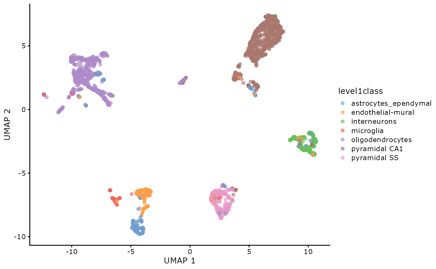
Dimensionality Reduction in CAbiNet
The dimensionality reduction in CAbiNet is performed with
Correspondence Analysis (CA) by the package APL. The most
important parameters in the dimensionality reduction step are the number
of dimensions (dims) you want to keep (similar with the
number of principal components in PCA) and the number of genes
(top) with the highest inertia you want to keep.
top is set to 5000 by default, in which case the top 5000
genes with highest inertia will be selected before performing CA. If you
already picked the most highly variable genes in advance (as we did
above), you can keep all genes in the count matrix which will be handed
to the function.
The number of genes kept should not be set too low, as otherwise important marker genes are often removed from the data.
# Correspondence Analysis
caobj <- cacomp(
  sce[top_genes, ],
  assay = "logcounts",
  dims = 40,
  top = nrow(sce[top_genes, ]),
  python = TRUE
)
The parameter python = TRUE indicates that the singular
value decomposition in CA is performed with a pytorch implementation.
This can drastically speed up the computation, in particular for large
datasets. If you did not install all python dependencies for APL, please
set it to FALSE.
CAbiNet Biclustering
CAbiNet builds up a shared-nearest-neighbour (SNN) gene-cell graph
based on the dimensionality reduced CA space. To build up the graph, you
need to specify the number of nearest neighours (NNs) of cells and genes
in the function caclust with the parameter k.
As the cell-gene graph is made up of 4 sub-graphs (cell-cell, gene-gene,
cell-gene and gene-cell graph), there are also 4 different
ks that can be tuned. If k is set to a single
integer, CAbiNet will use the same k for all 4 sub-graphs. If, however,
a vector of 4 integers is supplied, it will use them as k
for the cell-cell, gene-gene, cell-gene and gene-cell graph in that
exact order. So, for example k = 30 is equivalent to
k = (30, 30, 30, 30), but
k = c(30, 15, 30, 30) uses a k half as large as for the
other graphs for the gene-gene graph. In our experience, setting k for
the gene-gene graph to approx. half of the other graphs leads to a good
visualization/biclustering. See also ?caclust.
The simplest way to run CAbiNet is therefore:
# SNN graph & biclustering
cabic <- caclust(
  obj = caobj,
  k = c(70, 35, 70, 70),
  select_genes = FALSE,
  algorithm = "leiden",
  resolution = 1
)
If a large number of genes have been kept during pre-processing, the
biMAP can become too crowded and it can be hard to identify marker genes
of interest. CAbiNet therefore includes a method to remove genes that do
not add much information to the biMAP. The paramter
select_genes indicates whether genes that have no edge to
any cell should be removed from the graph:
# SNN graph & biclustering
cabic <- caclust(
  obj = caobj,
  k = c(70, 35, 70, 70),
  select_genes = TRUE,
  prune_overlap = FALSE,
  algorithm = "leiden",
  resolution = 1
)
Furthermore, we offer an optional graph pruning procedure with
parameters prune_overlap and overlap to remove
sporadic edges between cells and genes. Setting
prune_overlap as TRUE and overlap
as a fraction between 0 and 1 allows you to trim out edges between cells
and genes that are shared with less than ‘overlap’-fraction cell
neighours. Note this function only works when select_genes
is set as TRUE.
In many cases we also have a set of marker genes that we would like
to use for cell type annotation. In order to prevent the marker genes to
be removed during the graph pruning we can make the algorithm aware of
them using the marker_genes parameter.
# Marker genes from A. Zeisel et al., Cell types in the mouse cortex and hippocampus revealed by single-cell RNA-seq, 2015, Science
markers <- c(
  "Gad1",
  "Tbr1",
  "Spink8",
  "Mbp",
  "Aldoc",
  "Aif1",
  "Cldn5",
  "Acta2"
)

# SNN graph & biclustering
cabic <- caclust(
  obj = caobj,
  k = c(70, 35, 70, 70),
  select_genes = TRUE,
  prune_overlap = TRUE,
  mode = "all",
  overlap = 0.2,
  algorithm = "leiden",
  leiden_pack = "igraph",
  resolution = 1,
  marker_genes = markers
)
After building the cell-gene graph, the biclustering is performed
with either the Leiden algorithm (algorithm = "leiden") or
Spectral clustrering (algorithm = "spectral"). For the
up-to-date version of the package, we call the “leiden” function from
either the R package leiden or igraph. The
igraph implementation can be applied by set “leiden_pack =
‘igraph’” (as default, see ?caclust). From our testing, the
igraph implementation runs faster than package leiden
with similar accuracy. Therefore, we recommend to set
leiden_pack = "igraph".
The resulting caclust object contains biclustering results and the SNN graph:
cabic
#> caclust object with 2874 cells and 1617 genes.
#> 8 clusters found.
#> Clustering results:
#>
#>  cluster ncells ngenes
#>  1       297    154
#>  2        34     68
#>  3       440    144
#>  4       242    185
#>  5       846    237
#>  6       146    187
#>  7       597    317
#>  8       272    325
The cluster assignments for the cells or genes can be obtained with
the functions gene_clusters() and
cell_clusters():
sce$cabinet <- cell_clusters(cabic)

cat("Gene clusters:\n")
head(gene_clusters(cabic))

cat("\nCell clusters:\n")
head(cell_clusters(cabic))
#> Gene clusters:
#>   Apod    Mog   Ermn  Ptgds Opalin   Aspa
#>      7      7      7      7      7      7
#> Levels: 1 2 3 4 5 6 7 8
#>
#> Cell clusters:
#> 1772071015_C02 1772071017_G12 1772071017_A05 1772071014_B06 1772067065_H06
#>              1              1              1              1              1
#> 1772071017_E02
#>              1
#> Levels: 1 2 3 4 5 6 7 8
If too many genes are included in the graph, CAbiNet may detect some clusters which only contain genes. These genes probably are not marker genes and do not help in annotating the cells. We can therefore safely remove these mono-clusters by running:
cabic <- rm_monoclusters(cabic)
cabic
#> caclust object with 2874 cells and 1617 genes.
#> 8 clusters found.
#> Clustering results:
#>
#>  cluster ncells ngenes
#>  1       297    154
#>  2        34     68
#>  3       440    144
#>  4       242    185
#>  5       846    237
#>  6       146    187
#>  7       597    317
#>  8       272    325
As in this example there weren’t any mono-clusters, the results are identical to what we saw before. Removing monoclusters should be done before computing the biMAP. As an added benefit, removing the mono-clusters often improves the layout of the embedding.
Visualization of cells and genes in the biMAP
We now compute the biMAP embedding and visualize it in a scatter plot:
# Compute biMAP embedding.
cabic <- biMAP(cabic, k = 30)
# plot results
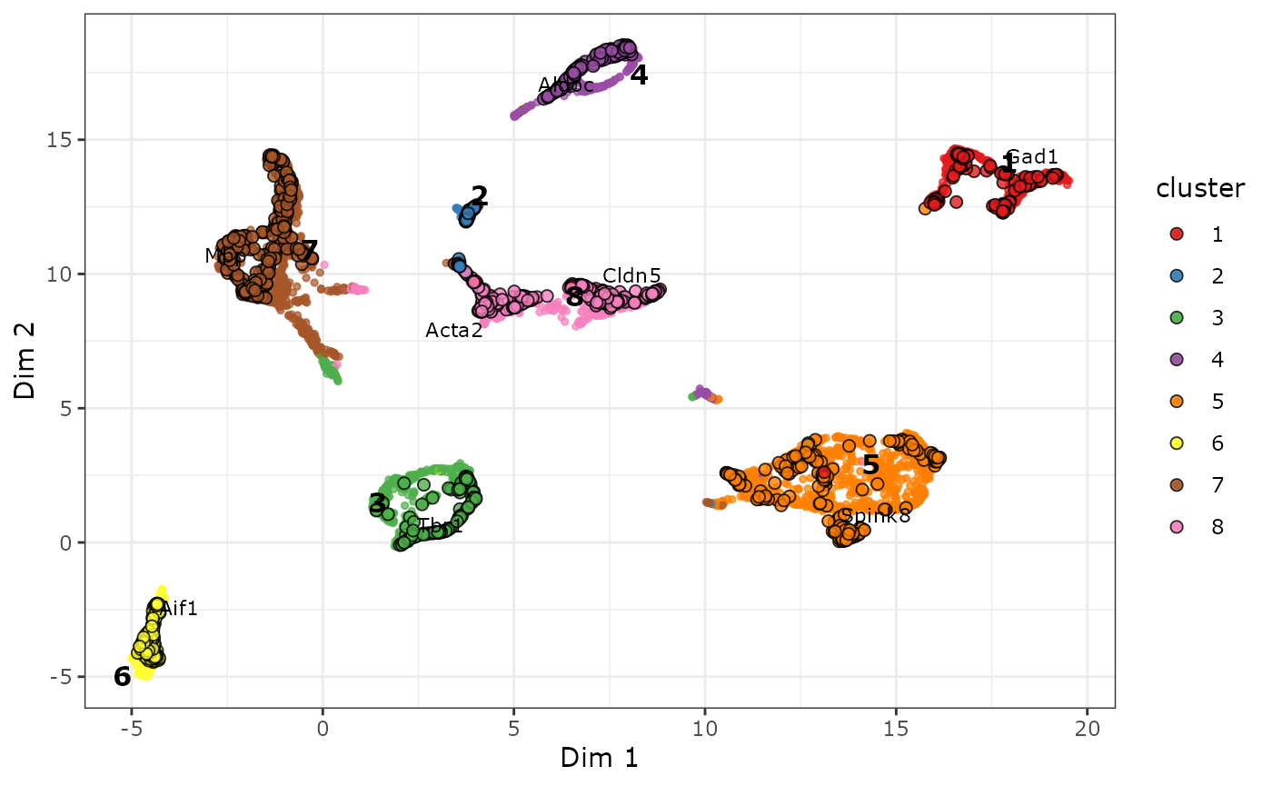
plot_biMAP(cabic,
color_genes = TRUE,
label_marker_genes = markers
)
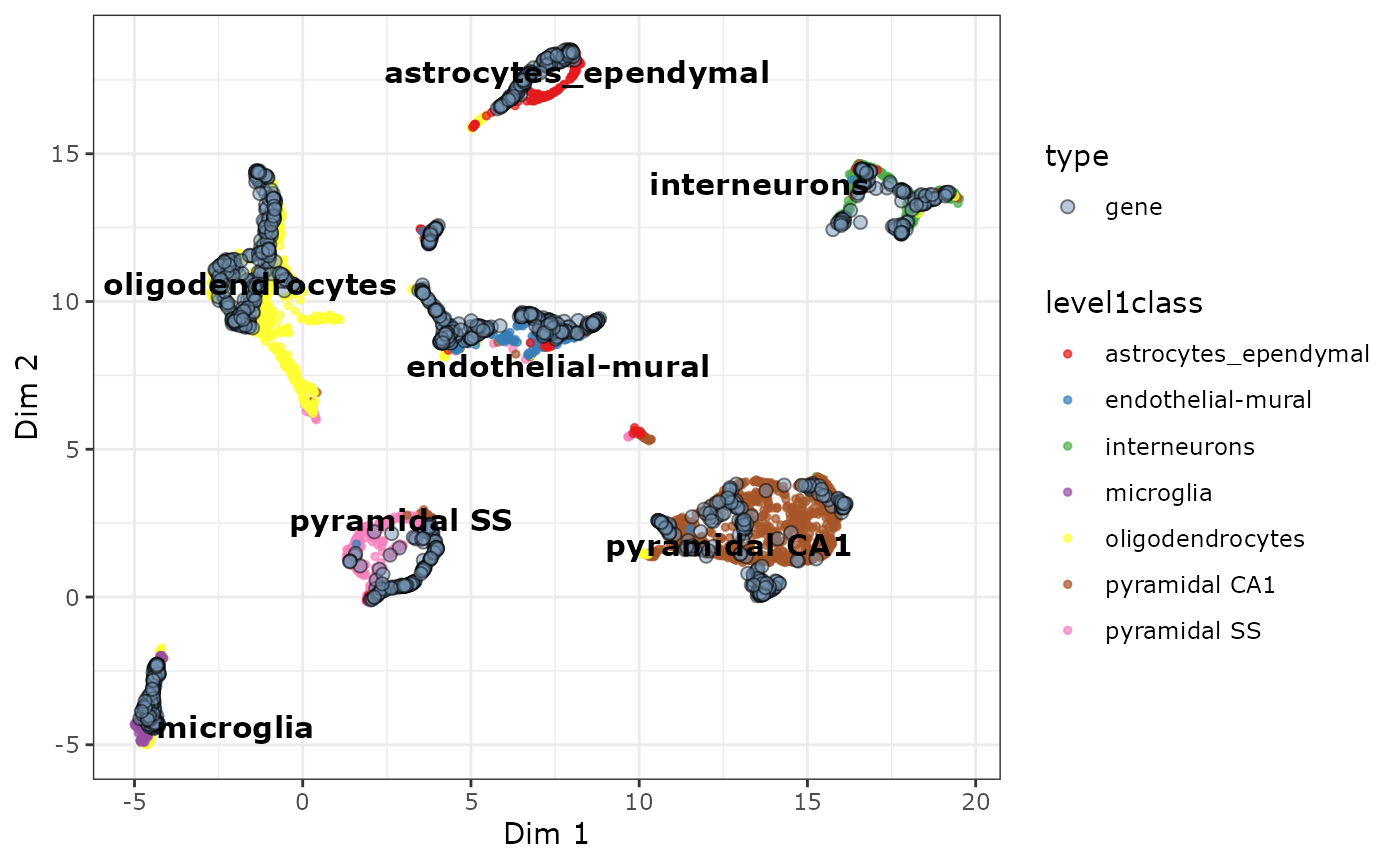
# only plot the cell clusters
plot_scatter_biMAP(cabic,
  gene_alpha = 0.5,
  color_genes = FALSE,
  color_by = "level1class",
  meta_df = colData(sce)
)
plot_biMAP and plot_scatter_biMAP both
produce a scatter plot of the embedding. For very large data sets it can
become difficult to differentiate between cells and genes in such a
plot. If we are mainly interested in identifying the marker genes of the
clusters, we can instead use the hex biMAP for a less busy
visualization:
plot_hex_biMAP(cabic, color_genes = TRUE, hex_n = 20)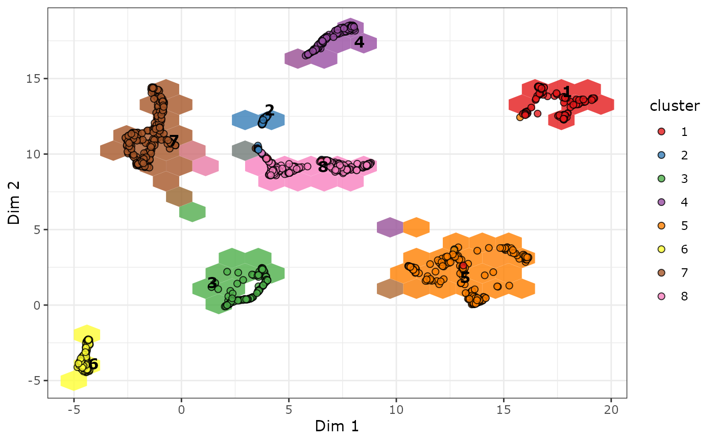
Cell type annotation
CAbiNet allows for intuitive cell type annotation. Instead of having to make a large number of feature plots, we can simply display the position of a set of marker genes directly in the biMAP. By the position of genes and cells in the biMAP, we can easily tell the marker genes of each cell group without having to perform differential gene expression analysis.
cts <- c(
  "Interneurons",
  "S1 Pyramidal",
  "CA 1 Pyramidal",
  "Oligodendrocytes",
  "Astrocytes",
  "Microglia",
  "Endothelial",
  "Mural"
)

## make sure the cell types and marker genes are in a one-to-one order.
df <- data.frame(
  cell_type = cts,
  marker_gene = markers
)

genecls <- gene_clusters(cabic)
biclusters <- vector(mode = "numeric", length = nrow(df))

for (i in seq_along(df$marker_gene)) {
  biclusters[i] <- genecls[df$marker_gene[i]]
}

df$cabinet <- biclusters
df
#>          cell_type marker_gene cabinet
#> 1     Interneurons        Gad1       1
#> 2     S1 Pyramidal        Tbr1       3
#> 3   CA 1 Pyramidal      Spink8       5
#> 4 Oligodendrocytes         Mbp       7
#> 5       Astrocytes       Aldoc       4
#> 6        Microglia        Aif1       6
#> 7      Endothelial       Cldn5       8
#> 8            Mural       Acta2       8
sce$cabinet_ct <- as.numeric(sce$cabinet)

for (i in seq_along(df$cabinet)) {
  sel <- which(sce$cabinet_ct == df$cabinet[i])
  sce$cabinet_ct[sel] <- df$cell_type[i]
}
sce$cabinet_ct <- as.factor(sce$cabinet_ct)

plot_biMAP(cabic,
  meta_df = colData(sce),
  color_by = "cabinet_ct",
  label_marker_genes = markers,
  color_genes = FALSE
)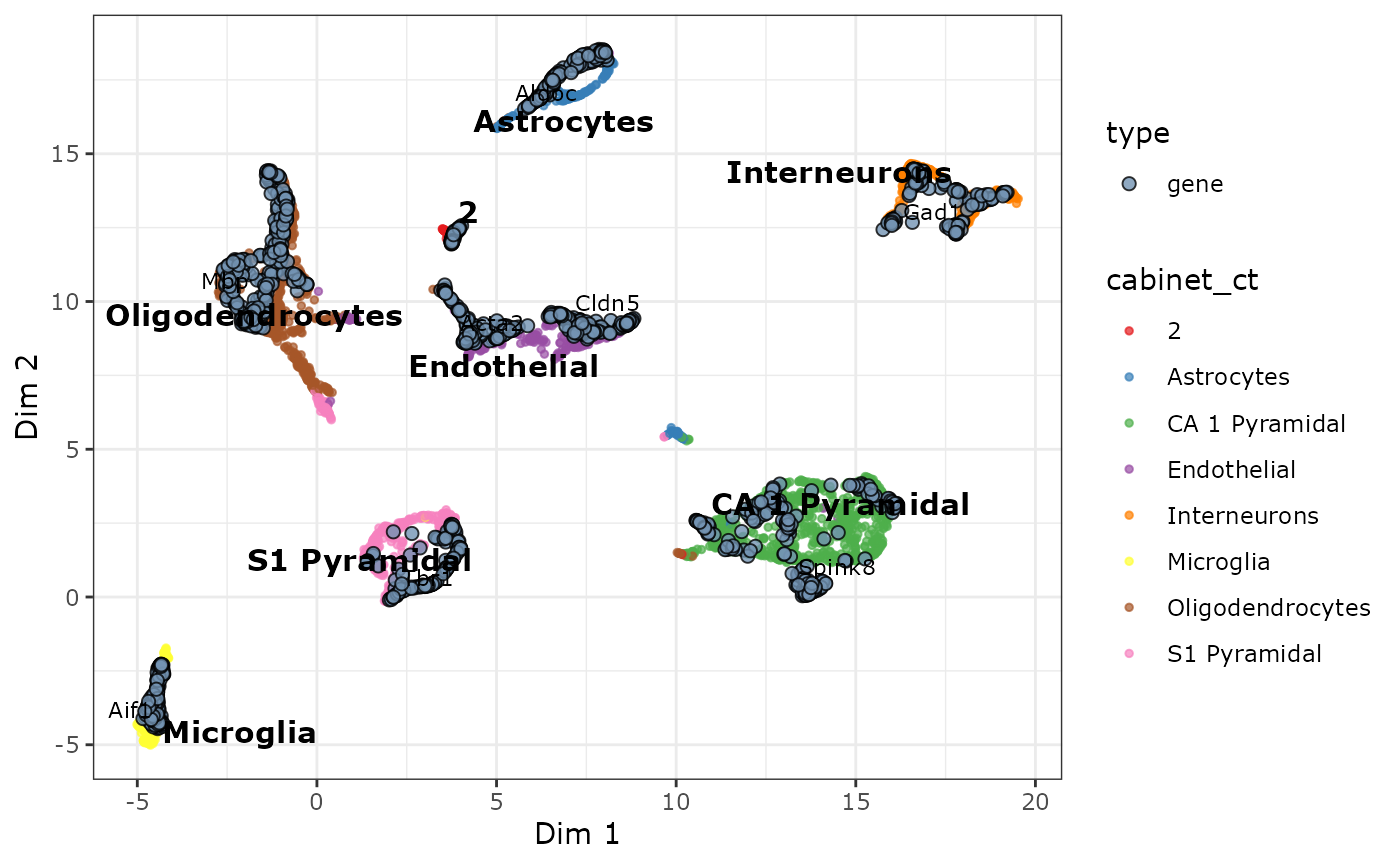
The only remaining unnanotated cluster is bicluster 2. This cluster consists mostly of cells that have been annotated as astrocytes, but also oligodendrocytes and pyramidal CA1 cells. It could be that this is a either a distinct sub-cell type or a group of outliers/doublets. We can also see the similar cell types Endothelial and Mural have been clustered in a single cluster (labelled Endothelial).
Using a feature biMAP to visualize the expression of the two Marker genes Acta2 (Mural) and Cldn5 (Endothelial) we can confirm that this cluster could be further subdivided by the location of the marker genes.
p1 <- plot_feature_biMAP(
  sce = sce,
  caclust = cabic,
  feature = "Acta2",
  label_size = 4
)

p2 <- plot_feature_biMAP(
  sce = sce,
  caclust = cabic,
  feature = "Cldn5",
  label_size = 4
)

p1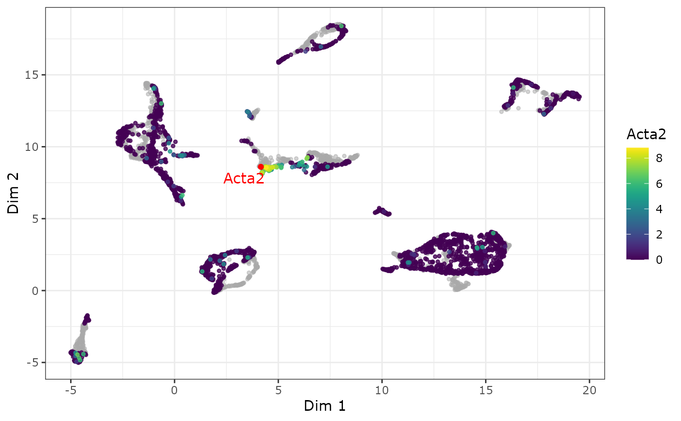
p2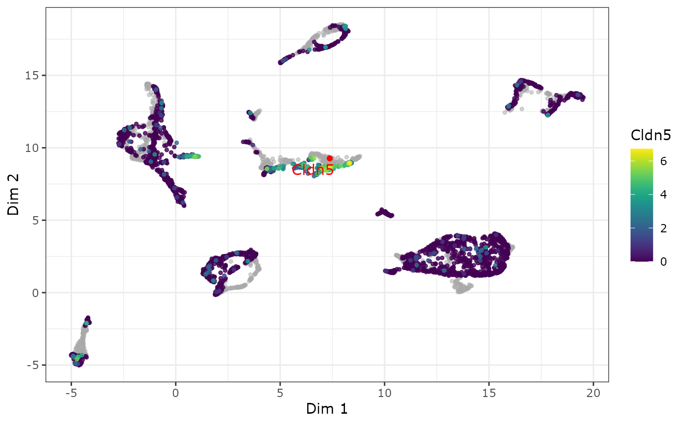
If you do not have a list of known marker genes for the cell types in
your data, you can use the annotate_biclustering()
function. It uses the “CellMarker” gene set to automatically annotate
the biclusters with the best matching cell type in the set:
ann_cabic <- annotate_biclustering(
  obj = cabic,
  universe = rownames(sce),
  org = "mm",
  set = "CellMarker"
)

plot_biMAP(
  ann_cabic,
  color_genes = TRUE,
  label_marker_genes = markers
)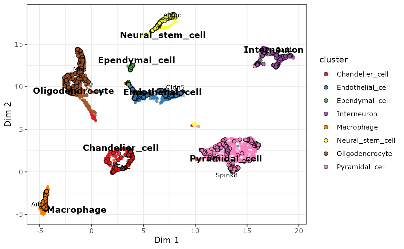
Last but not least, you can explore the visualization interactively, or just display the names of the marker genes in the plot. Co-clustered genes can be labeled in the biMAP. For example, if you don’t have a list of known marker genes at hand, you can display the names of potential marker genes by
plot_biMAP(
  cabic,
  color_by = "cluster",
  label_marker_genes = TRUE,
  group_label_size = 6,
  color_genes = TRUE,
  max.overlaps = 40
)
#> Warning: ggrepel: 1617 unlabeled data points (too many overlaps). Consider
#> increasing max.overlaps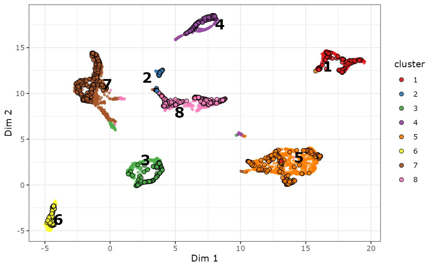
Sometimes the name of genes overlap with each other and can be difficult to read the names in the plot. Exploring the biMAP interactively allows you to zoom in or out at a group of points to inspect the information there in more detail:
plot_biMAP(cabic,
  color_by = "cluster",
  color_genes = TRUE,
  interactive = TRUE
)
#> Warning in geom2trace.default(dots[[1L]][[1L]], dots[[2L]][[1L]], dots[[3L]][[1L]]): geom_GeomTextRepel() has yet to be implemented in plotly.
#>   If you'd like to see this geom implemented,
#>   Please open an issue with your example code at
#>   https://github.com/ropensci/plotly/issues
Integration with Bioconductor packages
When intergrating the clustering results and cell type annotations with the SCE object, gene expression levels can also be visualized by violin plots.
scater::plotExpression(sce,
  features = markers[markers %in% rownames(sce)],
  x = "cabinet", colour_by = "cabinet"
) +
  theme(axis.text.x = element_text(angle = 0, hjust = 1))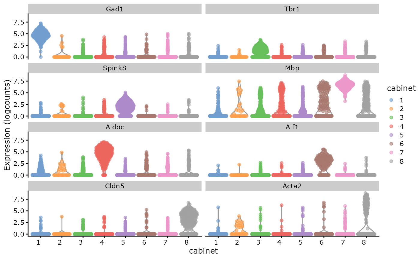
scater::plotExpression(sce,
features = markers[markers %in% rownames(sce)],
x = "level1class", colour_by = "level1class"
) +
theme(axis.text.x = element_text(angle = 30, hjust = 1))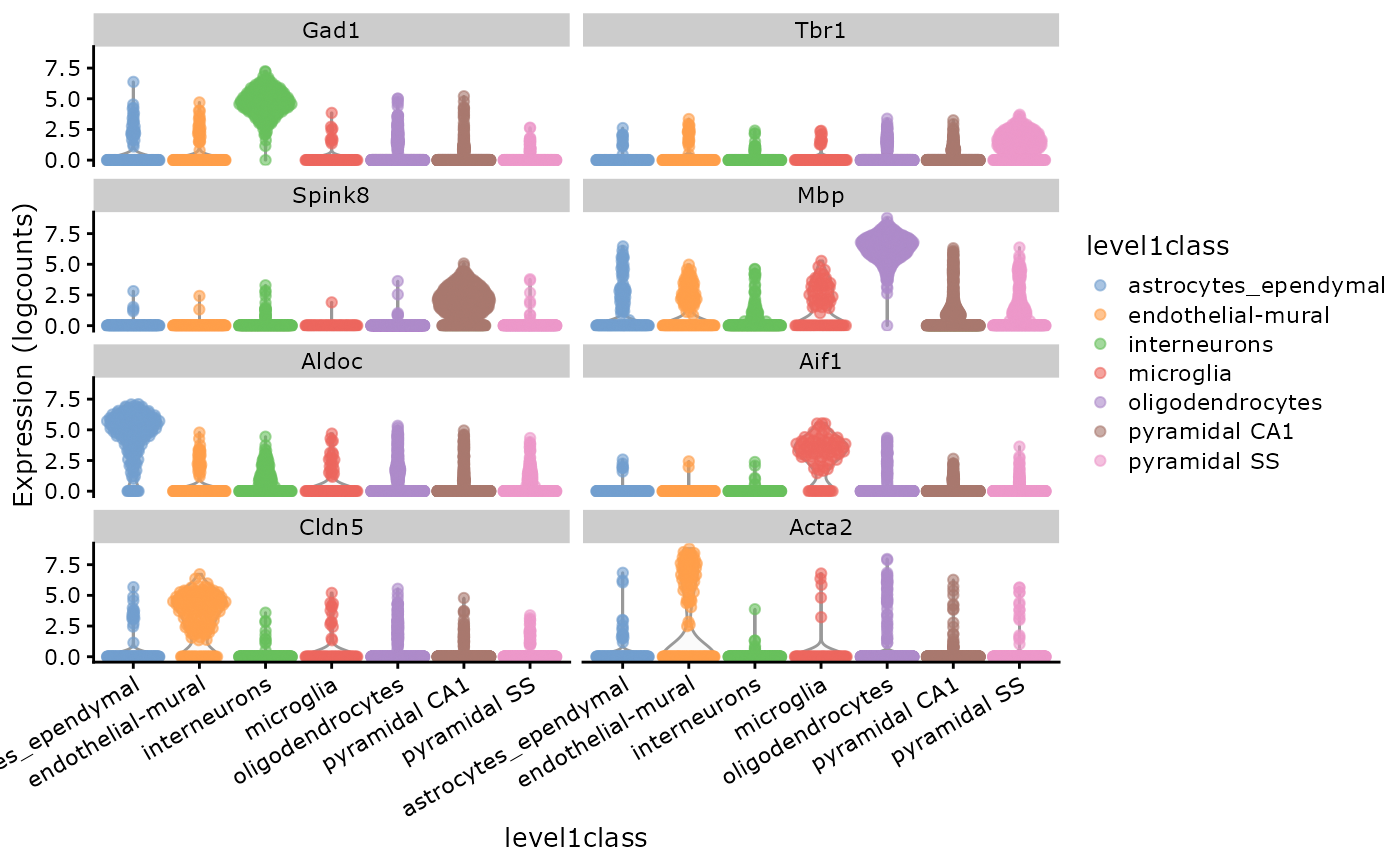 Since CAbiNet only co-clusters the up-regulated genes with cell groups,
the information of down-regulated genes is missing. To find out all the
dysregulated genes, you can make use of the cell clustering results from
CAbiNet and differential gene expression results from other packges to
study the dysregulated genes for different cell clusters.
Since CAbiNet only co-clusters the up-regulated genes with cell groups,
the information of down-regulated genes is missing. To find out all the
dysregulated genes, you can make use of the cell clustering results from
CAbiNet and differential gene expression results from other packges to
study the dysregulated genes for different cell clusters.
Session info
#> R version 4.2.1 (2022-06-23)
#> Platform: x86_64-pc-linux-gnu (64-bit)
#> Running under: MarIuX64 2.0 GNU/Linux
#>
#> Matrix products: default
#> BLAS:   /pkg/R-4.2.1-0/lib/R/lib/libRblas.so
#> LAPACK: /home/kohl/.local/share/r-miniconda/envs/r-reticulate/lib/libmkl_intel_lp64.so
#>
#> locale:
#>  [1] LC_CTYPE=en_US.UTF-8 LC_NUMERIC=C         LC_TIME=C
#>  [4] LC_COLLATE=C         LC_MONETARY=C        LC_MESSAGES=C
#>  [7] LC_PAPER=C           LC_NAME=C            LC_ADDRESS=C
#> [10] LC_TELEPHONE=C       LC_MEASUREMENT=C     LC_IDENTIFICATION=C
#>
#> attached base packages:
#> [1] stats4    stats     graphics  grDevices utils     datasets  methods
#> [8] base
#>
#> other attached packages:
#>  [1] scater_1.24.0               ggplot2_3.5.0
#>  [3] scran_1.24.1                scuttle_1.6.3
#>  [5] scRNAseq_2.10.0             SingleCellExperiment_1.18.1
#>  [7] SummarizedExperiment_1.26.1 Biobase_2.58.0
#>  [9] GenomicRanges_1.48.0        GenomeInfoDb_1.34.9
#> [11] IRanges_2.32.0              S4Vectors_0.36.2
#> [13] BiocGenerics_0.44.0         MatrixGenerics_1.8.1
#> [15] matrixStats_0.62.0          CAbiNet_0.99.2
#> [17] APL_1.2.0                   BiocStyle_2.24.0
#>
#> loaded via a namespace (and not attached):
#>   [1] rappdirs_0.3.3                SparseM_1.81
#>   [3] rtracklayer_1.56.1            scattermore_0.8
#>   [5] SeuratObject_4.1.0            ragg_1.2.2
#>   [7] tidyr_1.3.1                   bit64_4.0.5
#>   [9] knitr_1.46                    irlba_2.3.5.1
#>  [11] DelayedArray_0.22.0           data.table_1.15.4
#>  [13] rpart_4.1.16                  KEGGREST_1.38.0
#>  [15] RCurl_1.98-1.8                AnnotationFilter_1.20.0
#>  [17] generics_0.1.3                GenomicFeatures_1.48.3
#>  [19] org.Mm.eg.db_3.15.0           ScaledMatrix_1.4.0
#>  [21] cowplot_1.1.3                 RSQLite_2.3.6
#>  [23] RANN_2.6.1                    future_1.27.0
#>  [25] bit_4.0.5                     spatstat.data_3.0-4
#>  [27] xml2_1.3.3                    httpuv_1.6.5
#>  [29] assertthat_0.2.1              viridis_0.6.5
#>  [31] xfun_0.43                     hms_1.1.1
#>  [33] jquerylib_0.1.4               evaluate_0.15
#>  [35] promises_1.2.0.1              additivityTests_1.1-4.1
#>  [37] fansi_1.0.6                   restfulr_0.0.15
#>  [39] progress_1.2.2                dbplyr_2.2.1
#>  [41] igraph_2.0.3                  DBI_1.2.2
#>  [43] htmlwidgets_1.5.4             spatstat.geom_3.2-9
#>  [45] purrr_1.0.2                   ellipsis_0.3.2
#>  [47] crosstalk_1.2.0               RSpectra_0.16-1
#>  [49] dplyr_1.1.4                   bookdown_0.27
#>  [51] biomaRt_2.52.0                deldir_1.0-6
#>  [53] sparseMatrixStats_1.8.0       vctrs_0.6.5
#>  [55] here_1.0.1                    ensembldb_2.20.2
#>  [57] ROCR_1.0-11                   abind_1.4-5
#>  [59] withr_3.0.0                   cachem_1.0.8
#>  [61] RcppEigen_0.3.4.0.0           progressr_0.10.1
#>  [63] sctransform_0.3.3             GenomicAlignments_1.32.1
#>  [65] prettyunits_1.1.1             goftest_1.2-3
#>  [67] cluster_2.1.3                 ExperimentHub_2.4.0
#>  [69] lazyeval_0.2.2                crayon_1.5.2
#>  [71] labeling_0.4.3                edgeR_3.38.2
#>  [73] pkgconfig_2.0.3               vipor_0.4.5
#>  [75] nlme_3.1-158                  ProtGenerics_1.28.0
#>  [77] rlang_1.1.3                   globals_0.15.1
#>  [79] lifecycle_1.0.4               miniUI_0.1.1.1
#>  [81] filelock_1.0.2                BiocFileCache_2.4.0
#>  [83] rsvd_1.0.5                    AnnotationHub_3.4.0
#>  [85] rprojroot_2.0.3               polyclip_1.10-6
#>  [87] lmtest_0.9-40                 graph_1.74.0
#>  [89] Matrix_1.5-4                  zoo_1.8-10
#>  [91] beeswarm_0.4.0                ggridges_0.5.3
#>  [93] png_0.1-8                     viridisLite_0.4.2
#>  [95] rjson_0.2.21                  bitops_1.0-7
#>  [97] KernSmooth_2.23-20            Biostrings_2.66.0
#>  [99] blob_1.2.4                    DelayedMatrixStats_1.18.2
#> [101] stringr_1.5.1                 parallelly_1.32.1
#> [103] spatstat.random_3.2-3         beachmat_2.12.0
#> [105] scales_1.3.0                  hexbin_1.28.2
#> [107] memoise_2.0.1                 magrittr_2.0.3
#> [109] plyr_1.8.9                    ica_1.0-3
#> [111] zlibbioc_1.44.0               compiler_4.2.1
#> [113] dqrng_0.3.0                   BiocIO_1.6.0
#> [115] RColorBrewer_1.1-3            fitdistrplus_1.1-8
#> [117] Rsamtools_2.12.0              cli_3.6.2
#> [119] XVector_0.38.0                listenv_0.8.0
#> [121] patchwork_1.2.0               pbapply_1.5-0
#> [123] MASS_7.3-58                   mgcv_1.8-40
#> [125] tidyselect_1.2.1              stringi_1.8.3
#> [127] RcppHungarian_0.3             textshaping_0.3.6
#> [129] highr_0.9                     yaml_2.3.5
#> [131] locfit_1.5-9.6                BiocSingular_1.12.0
#> [133] ggrepel_0.9.5                 grid_4.2.1
#> [135] sass_0.4.2                    tools_4.2.1
#> [137] future.apply_1.9.0            parallel_4.2.1
#> [139] bluster_1.6.0                 metapod_1.4.0
#> [141] gridExtra_2.3                 farver_2.1.1
#> [143] Rtsne_0.16                    digest_0.6.35
#> [145] BiocManager_1.30.22           rgeos_0.5-9
#> [147] FNN_1.1.4                     shiny_1.7.2
#> [149] flexclust_1.4-1               Rcpp_1.0.12
#> [151] BiocVersion_3.15.2            later_1.3.0
#> [153] RcppAnnoy_0.0.19              org.Hs.eg.db_3.15.0
#> [155] httr_1.4.7                    AnnotationDbi_1.60.2
#> [157] colorspace_2.1-0              biclust_2.0.3.1
#> [159] XML_3.99-0.10                 fs_1.6.3
#> [161] topGO_2.48.0                  tensor_1.5
#> [163] reticulate_1.25               splines_4.2.1
#> [165] statmod_1.4.36                uwot_0.1.11
#> [167] spatstat.utils_3.0-4          pkgdown_2.0.6
#> [169] sp_1.5-0                      plotly_4.10.4
#> [171] systemfonts_1.0.6             xtable_1.8-4
#> [173] jsonlite_1.8.8                modeltools_0.2-23
#> [175] R6_2.5.1                      pillar_1.9.0
#> [177] htmltools_0.5.3               mime_0.12
#> [179] glue_1.7.0                    fastmap_1.1.1
#> [181] BiocParallel_1.32.6           BiocNeighbors_1.14.0
#> [183] class_7.3-20                  interactiveDisplayBase_1.34.0
#> [185] codetools_0.2-18              utf8_1.2.4
#> [187] lattice_0.20-45               bslib_0.4.0
#> [189] spatstat.sparse_3.0-3         tibble_3.2.1
#> [191] ggbeeswarm_0.6.0              curl_5.2.1
#> [193] leiden_0.4.2                  GO.db_3.16.0
#> [195] limma_3.52.4                  survival_3.3-1
#> [197] rmarkdown_2.26                desc_1.4.1
#> [199] munsell_0.5.1                 GenomeInfoDbData_1.2.9
#> [201] reshape2_1.4.4                gtable_0.3.4
#> [203] spatstat.core_2.4-4           Seurat_4.1.1